View Transformer Layers from Online Optimization Perspective

Background: Linear Attention and State-space Model

We begin by reviewing the standard Transformer notation to set the stage for understanding linear attention and its relationship to state-space models (SSMs).

Given an input sequence $x_1, x_2, \ldots, x_T \in \mathbb{R}^D$, the attention layer maps each input token $x_t$ to a query $q_t = W_q x_t$, key $k_t = W_k x_t$, and value $v_t = W_v x_t$, where $W_q, W_k, W_v \in \mathbb{R}^{D \times D}$ are learned projection matrices. The output at time step $t$ is given by the standard softmax attention:

$$o_t = \sum_{j=1}^{t} \alpha_{tj} v_j, \quad \alpha_{tj} = \frac{\exp(q_t^\top k_j)}{\sum_{l=1}^{t} \exp(q_t^\top k_l)}. \tag{1}$$

This softmax-based formulation ensures that attention weights are positive and sum to one, allowing the model to selectively focus on relevant past information. While softmax attention is effective, its quadratic time and memory complexity with respect to sequence length $T$ becomes a bottleneck for long-context modeling. Linear attention addresses this by replacing the softmax with a kernel function $\phi(\cdot)$. In the simplest case, using $\phi(x) = x$ (i.e., identity function), the attention reduces to an unnormalized form:

$$o_t = \sum_{j=1}^{t} v_j \left( k_j^\top q_t \right) = \left( \sum_{j=1}^{t} v_j k_j^\top \right) q_t = S_t q_t. \tag{2}$$

Here, we define the matrix-valued hidden state $S_t \in \mathbb{R}^{d \times d}$ as the accumulated sum of outer products of past key and value vectors to get rid of the KV cache that grows with sequence length:

$$S_t := \sum_{j=1}^{t} v_j k_j^\top. \tag{3}$$

This formulation offers a key computational advantage: by exploiting the associativity of matrix-vector multiplication, we can compute the attention output at time $t$ using the current query vector $q_t$ and the pre-computed state matrix $S_t$, without explicitly iterating over all past tokens. Moreover, $S_t$ can be updated incrementally in constant time as new tokens arrive, following a rank-one update rule:

$$S_t = S_{t-1} + v_t k_t^\top. \tag{4}$$

Thus, linear attention transforms the original $O(T^2)$ attention mechanism into a recurrent-style process with $O(T)$ time complexity, where the model only needs to maintain and update a fixed-size $O(d^2)$ memory matrix $S_t$ over time.

Interestingly, this recurrent update in linear attention mirrors the update rule of certain state-space models. In general, an SSM is defined as:

$$h_t = A_t h_{t-1} + B_t x_t, \quad y_t = C_t h_t, \tag{5}$$

where $h_t$ is the hidden state, $x_t$ the input, and $y_t$ the output. This reveals that linear attention is not merely a Transformer variant—it is a specific instance of a state-space model, where memory is stored and updated through structured recurrence.

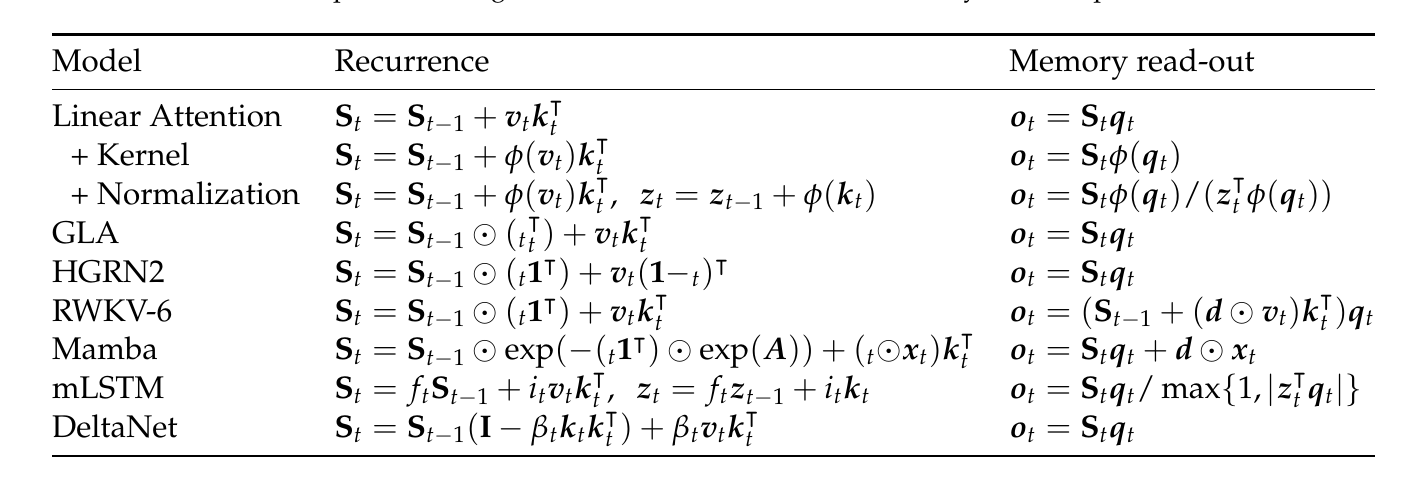
As shown in Table 1, we can formulate Linear Transformers and state-space models under a unified framework. Their main difference lies in how the hidden state $S$ is updated over time, as well as how it interacts with new queries.

Fast Weight Programming

Fast weights provide a neurally plausible way of implementing the type of temporary storage that is required by working memory, while slow weights capture more permanent associations learned over many experiences.

Geoffrey Hinton

In this view, the hidden state $S_t$ serves as a form of fast weights that are rapidly updated at each time step to store temporary associations from recent inputs. These fast weights are distinct from the slow weights (e.g., $W_q, W_k, W_v$, or transition matrices $A, B, C$ in SSMs), which are learned parameters updated during training and shared across the entire sequence.

We revisit the update rule for the hidden state $S$ in the simplest form of linear attention:

$$S_t = S_{t-1} + v_t k_t^\top.$$

If we consider $S_t$ as an updated weight, we first define a simple objective function at time step $t$:

$$\mathcal{L}_t(S) = -\langle S k_t, v_t \rangle. \tag{6}$$

This objective encourages $S$ to transform $k_t$ into a vector that is well aligned with $v_t$. Taking the gradient of this loss with respect to $S$ gives:

$$\nabla \mathcal{L}_t(S) = -v_t k_t^\top. \tag{7}$$

A single step of stochastic gradient descent (SGD) on this loss yields the update rule:

$$S_t = S_{t-1} - \beta_t \nabla \mathcal{L}_t(S_{t-1}) = S_{t-1} + \beta_t v_t k_t^\top, \tag{8}$$

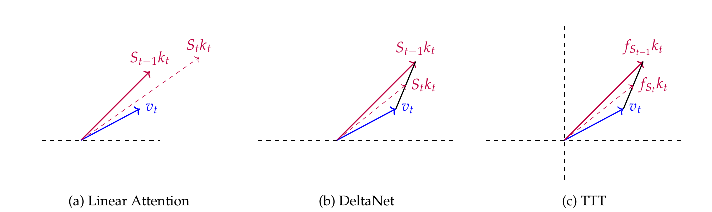
where $\beta_t$ is a learning rate that controls the step size of the update. In standard linear attention, this is implicitly set to $\beta_t = 1$, and it just the form in Equation 4. As shown in Fig. 2 (a), this corresponds to minimizing the angle between them and increasing the magnitude of $S_t k_t$. In essence, it adjusts the response along the direction of $k_t$ so that it better aligns with $v_t$. This way, when a similar key vector appears in the future, the memory matrix $S$ will produce an output that is more aligned with the previously observed value $v_t$. The model incrementally learns the association “if you see $k_t$, then output $v_t$,” embedding this knowledge into the fast weights.

An alternative formulation proposed by [4] shown in Fig. 2 (b) is to directly minimize the squared Euclidean distance between the predicted output $S k_t$ and the ground-truth target $v_t$:

$$\mathcal{L}_t(S) = \frac{1}{2}\| S k_t - v_t \|^2 \tag{9}$$

The gradient of this loss with respect to $S$ is:

$$\nabla \mathcal{L}_t(S) = (S k_t - v_t) k_t^\top \tag{10}$$

This leads to the following update rule via stochastic gradient descent:

$$S_t = S_{t-1} - \beta_t \nabla \mathcal{L}_t(S_{t-1}) = S_{t-1} - \beta_t (S_{t-1} k_t - v_t) k_t^\top \tag{11}$$

If we further apply $L_2$ normalization to $k_t$, as is done in [4], so that $k_t^\top k_t = 1$, Equation 11 simplifies to:

$$S_t k_t = S_{t-1} k_t - \beta_t \left( S_{t-1} k_t - v_t \right) = (1 - \beta_t) S_{t-1} k_t + \beta_t v_t. \tag{12}$$

In other words, the output $S_t k_t$ is obtained by linearly interpolating between the previously retrieved value $S_{t-1} k_t$ and the new target value $v_t$, controlled by the update rate $\beta_t$. Geometrically, as illustrated in Fig. 2 (b), this means that $S_{t-1} k_t$, $S_t k_t$, and $v_t$ all lie on the same line, forming a convex combination. From the perspective of key-value retrieval, this formulation suggests that we first retrieve the “old value” associated with $k_t$ from $S_{t-1}$, and adjust it towards the new observation $v_t$. This type of state update mechanism, proposed in [1], is referred to as “Delta Rule”.

Test-Time Training (TTT) [2] further generalizes the fast weight perspective by treating the hidden state $S_t$ not merely as a memory matrix, but as the parameters of a learnable model that evolves via gradient descent on a self-supervised objective during inference.

Equation 6 and 9 assumes a linear relationship between the key $k_t$ and target $v_t$ since the only modeling term is the state matrix $S$. While computationally efficient, such a formulation limits the expressivity needed to capture complex, nonlinear dependencies tasks. TTT lifts this limitation by modeling $S_t$ as the parameters of a learnable function $f_{S_t}$, and updating it via online gradient descent:

$$\mathcal{L}_t(f_S) = \frac{1}{2}\| f_S(k_t) - v_t \|^2. \tag{13}$$

In a sense, TTT also can be viewed as a parametric and learnable generalization of kernelized linear attention—replacing fixed feature maps with gradient-updated neural learners.

TTT proposes two instantiations of the function $f_S$, each capturing a different level of model expressivity:

$$\textbf{TTT-Linear}: \quad f_S(x) = \mathrm{LN}(\mathrm{Linear}(x)) + x \tag{14}$$

Here, $\mathrm{LN}(\cdot)$ denotes layer normalization. While the core transformation $\mathrm{Linear}(x)$ is linear, the inclusion of layer normalization introduces a form of nonlinearity.

$$\textbf{TTT-MLP}: \quad f_S(x) = \mathrm{LN}(\mathrm{MLP}(x)) + x, \quad \text{where} \quad \mathrm{MLP}(x) = W_2\, \sigma(W_1 x) \tag{15}$$

In this case, $f_S$ is a two-layer feedforward network with GeLU activation $\sigma$, mirroring the architecture of MLP blocks in Transformer with an intermediate hidden dimension typically expanded by a factor of 4. In both variants, the parameters $S$ define a per-sequence learner that is continually updated at test time via gradient descent. This allows the model to adaptively encode fine-grained token-level associations—effectively learning “on the fly” from the input sequence.

Mesa-optimization

In the above discussion, we considered how the state updates in linear transformers during sequence modeling tasks can be viewed as an online optimization process. This optimization occurs along the sequence dimension, meaning that each time a new token is added, the state is updated once.

Mesa Layer [3] advances this view by proposing that Transformers implicitly implement a more general in-context learning algorithm—without being explicitly trained for it. They hypothesize that next-token prediction training installs an internal optimization loop that iteratively updates a latent predictor $f_S$ during inference. Specifically, for linear sequence modeling tasks, the goal is to find a predictor $f_S$ such that:

$$f_S = \arg\min_{f_S} \sum_{t=1}^{T-1} \frac{1}{2}\| f_S(k_t) - v_t \|^2 + \frac{\lambda}{2}\| f_S \|_F^2, \tag{16}$$

where $\lambda$ is a regularization constant. They made a bold methodological shift: rather than relying on gradient descent as in prior work, the Mesa layer analytically derives a closed-form solution of this ridge regression:

$$f_S = \left( \sum_{t=1}^{T-1} v_t k_t^\top \right) \left( \sum_{t=1}^{T-1} k_t k_t^\top + \lambda I \right)^{-1}. \tag{17}$$

There are two perspectives to understand how mesa-optimization unfolds inside a Transformer:

• Step-wise (temporal) view: At each time step $t$, the model updates an internal predictor $f_S$ based on all previous input-target pairs $\{(k_{t'}, v_{t'})\}_{t' < t}$, producing an output $o_t = f_S q_t$. This corresponds to performing close-form solution per new token, progressively refining the in-context predictor $f_S$ as the sequence grows.
• Layer-wise (depth) view: For a fixed token $t$, successive layers of the Transformer refine the token’s internal representation. In this view, each layer executes a portion of the optimization algorithm, so that after passing through each layer, the model has constructed a well-optimized $f_S$ suitable for predicting $v_t$ from $k_t$.

Both views are simultaneously valid. Along the sequence (step-wise), new tokens provide new supervision. Along the depth (layer-wise), the model iteratively processes each token’s local context to optimize and apply $f_S$. This unified dynamic effectively turns Transformer inference into an online optimizer over layers and time.

In practice, the Equation 17 enables an efficient per-token update through recursive least squares. By maintaining the inverse covariance matrix $R_t \in \mathbb{R}^{d \times d}$:

$$R_t = R_{t-1} - \frac{R_{t-1} k_t k_t^\top R_{t-1}}{1 + k_t^\top R_{t-1} k_t}, \quad R_0 = \lambda^{-1} I, \tag{18}$$

the predictor $f_S$ can be updated incrementally:

$$f_S = \left( \sum_{j=1}^{t} v_j k_j^\top \right) R_t. \tag{19}$$

The final attention output becomes:

$$o_t = f_S q_t = \left( \sum_{j=1}^{t} v_j k_j^\top \right) R_t q_t. \tag{20}$$

This recursive construction not only avoids quadratic complexity but also tightly integrates learning into the inference-time dynamics. Compared to the linear attention update $S_t = S_{t-1} + v_t k_t^\top$, which can be seen as a one-step gradient descent (as discussed in the fast weight section), the mesa-layer executes an exact least-squares fit over all previous key-value pairs. It transforms Transformer inference into a memory-efficient, online ridge regression solver that generalizes better across longer sequences and dynamic input distributions.

Discussion

While Transformer layers have been successfully interpreted as online optimizers in autoregressive language models, this perspective does not seamlessly transfer to Vision Transformers (ViTs) or Diffusion Transformers (DiTs), which operate on spatially unordered image patches and are trained without explicit token-level supervision or autoregressive masking. Despite the absence of a natural sequence or causal context, ViTs still exhibit strong performance across visual tasks. It raises the question: what kind of optimization, if any, unfolds across ViT layers?

One possible interpretation is that ViTs instantiate a depth-wise optimization process, where each layer serves not as a temporal update but as a refinement operator over a static input set. In MIM tasks, for example, the model receives corrupted images and gradually reconstructs missing patches by diffusing information across the token grid. Here, the notion of “optimization” is spatial and local: each patch token attends to others to iteratively improve a shared latent representation. Unlike the token-by-token predictor $f_S$ in language models, ViTs construct a global latent structure in a fully-parallel manner. The optimization process, if it exists, is implicitly encoded in the compositional transformations applied layer by layer.

Moreover, the absence of a causal mask in ViTs leads to a fundamentally different role for attention. Rather than computing sequence-conditioned updates, each token aggregates context from all other locations simultaneously, suggesting that ViTs function more like iterative solvers in graphical models—performing inference over a set of mutually dependent variables, rather than optimizing a unidirectional predictor. This depth-wise inference may resemble energy minimization or score matching, where each layer nudges the current state toward a lower-energy configuration aligned with the reconstruction or contrastive objective.

In short, while autoregressive Transformers clearly exhibit step-wise mesa-optimization dynamics, ViTs hint at a more spatially-distributed, depth-wise optimization process. Understanding whether this process can be made explicit—through layer-wise objectives, differentiable solvers, or architectural priors—could provide new insights into the inductive biases of Transformer architectures in vision.

Acknowledgments

We would like to thank the authors of all the papers referenced in this blog for their valuable contributions to advancing the field. In particular, we are grateful to Songlin Yang, whose notations and organization this post partially follows.

Citation

If you find this blog helpful, please cite:

@article{chaiview,
  title={View Transformer Layers from Online Optimization Perspective},
  author={Chai, Wenhao and Xu, Weili},
  year={2025},
  url={\url{https://wenhaochai.com/assets/file/blog/mesa.pdf}},
}

References

- Imanol Schlag, Kazuki Irie, and Jürgen Schmidhuber. Linear transformers are secretly fast weight programmers. arXiv preprint arXiv:2102.11174, 2021.
- Yu Sun, Xinhao Li, Karan Dalal, Jiarui Xu, Arjun Vikram, Genghan Zhang, Yann Dubois, Xinlei Chen, Xiaolong Wang, Sanmi Koyejo, et al. Learning to (learn at test time): RNNs with expressive hidden states. arXiv preprint arXiv:2407.04620, 2024.
- Johannes Von Oswald, Maximilian Schlegel, Alexander Meulemans, Seijin Kobayashi, Eyvind Niklasson, Nicolas Zucchet, Nino Scherrer, Nolan Miller, Mark Sandler, Max Vladymyrov, et al. Uncovering mesa-optimization algorithms in transformers. arXiv preprint arXiv:2309.05858, 2023.
- Songlin Yang, Bailin Wang, Yu Zhang, Yikang Shen, and Yoon Kim. Parallelizing linear transformers with the delta rule over sequence length. arXiv preprint arXiv:2406.06484, 2024.