The question
Hidden dimensions in a neural network are design choices: we pick a width, and the network fills it. The data itself never asked for that many coordinates, and networks are famously overparameterized relative to what their inputs require. The intrinsic dimension of a dataset is the number of variables needed in a minimal representation of the data: the smallest count of coordinates that still tells every sample apart along the directions where the data actually varies.
That raises a concrete question. Take ImageNet: 14 million images, more than 20,000 categories, each image stored at $224 \times 224$ resolution, which is 150,528 pixel values. The ambient dimension is in the hundreds of thousands. How many coordinates does the dataset truly use, and how would we measure that number from samples alone?
A toy contrast
Two scatter plots make the idea tangible. On the left, points drawn uniformly at random fill the unit square; no direction is privileged, and describing a point takes both coordinates. The intrinsic dimension matches the ambient dimension, two. On the right, correlated samples concentrate along one diagonal direction; a single coordinate along that axis captures most of the variation. PCA recovers exactly this kind of linear structure.
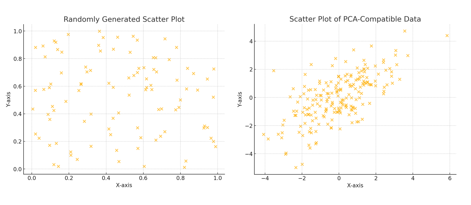
Natural images break the linear case: the set of plausible photographs is a curved, highly nonlinear subset of pixel space. The standard formalization is the manifold hypothesis, which treats the data as samples from a low-dimensional manifold embedded in the high-dimensional ambient space. Estimating intrinsic dimension then means estimating the dimension of that manifold without ever constructing it.
Setup
The estimator below, due to Levina and Bickel [1], needs only a notion of distance between samples. The setup:
- $P \subset \mathbb{R}^N$: the data points, living in an $N$-dimensional ambient space;
- $M \subseteq \mathbb{R}^N$: the manifold the data is sampled from;
- $m = \dim(M) \ll N$: the intrinsic dimension we want;
- local uniformity: density is treated as constant within small neighborhoods.
The MLE estimator
The key is a relationship between distance and dimension. Fix a data point and grow a ball of radius $r$ around it. Under local uniformity with density $\rho$, the expected number of neighbors inside the ball scales with its volume:
$$\mathbb{E}(\text{number of points}) = \rho V_m(r) \propto r^m,$$
where $V_m(r)$ is the volume of an $m$-dimensional ball, for instance $V_2(r) = \pi r^2$ and $V_3(r) = \tfrac{4}{3}\pi r^3$. The growth rate of neighbor counts in $r$ exposes $m$: in two dimensions doubling the radius quadruples the expected count, in three it octuples.
Levina and Bickel make this precise by modeling the process of observing neighbors at increasing distances $r_1, r_2, \ldots, r_k$ from the query point, the distances to its $k$ nearest neighbors, as an inhomogeneous Poisson process. The rate follows from differentiating the expected count:
$$\lambda(r) \propto \frac{d}{dr}\left[ r^m \right] = m \cdot r^{m-1},$$
and the probability of the observed process together with its log-likelihood are
$$P(N(r)) \propto \exp\left( -\int_0^R \lambda(r)\, dr \right) \prod_j \lambda(r_j), \qquad L(m) = \int_0^R \log \lambda(r)\, dN(r) - \int_0^R \lambda(r)\, dr.$$
Setting $\partial L / \partial m = 0$ gives a closed-form maximum likelihood estimate at each query point:
$$\hat{m} = \left[ \frac{1}{k-1} \sum_{j=1}^{k-1} \log \frac{r_k}{r_j} \right]^{-1},$$
where the neighbor count $k$ is the one hyperparameter. The estimate reads off how fast nearest-neighbor distances spread: when the ratios $r_k / r_j$ stay close to one, neighbors pack densely and the estimated dimension is low; when distances grow quickly, the data spreads through many directions and $\hat{m}$ rises. Averaging the per-point estimates over the dataset gives the global figure.
Sanity check on synthetic data
Does the estimator recover a dimension we control? Pope et al. [2] build a ground-truth testbed from a pretrained BigGAN with a 128-dimensional latent space: keep $\bar{d}$ latent coordinates free, zero out the rest, and the generated images form a manifold of known dimension $\bar{d}$ embedded in pixel space.
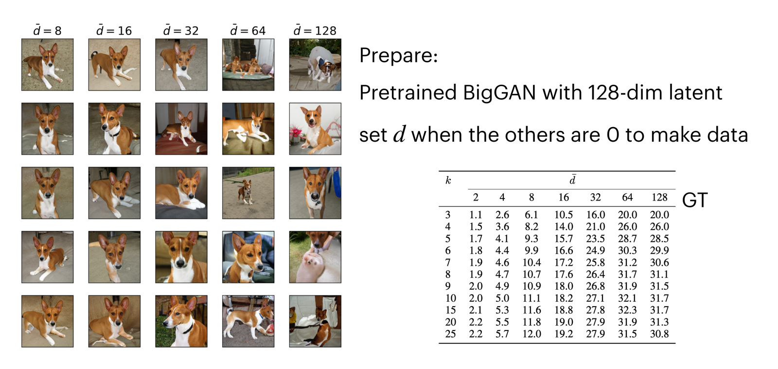
The estimates track the controlled dimension closely through $\bar{d} = 32$ and compress somewhat at 64 and 128. The tool is trustworthy in exactly the regime where natural image datasets turn out to live.
What real datasets measure
Applying the estimator to standard vision datasets produces the headline numbers. MNIST sits lowest, around 7 to 13 depending on $k$; CIFAR-10 and CelebA land in the teens to mid-twenties; ImageNet tops the chart at roughly 26 to 43.
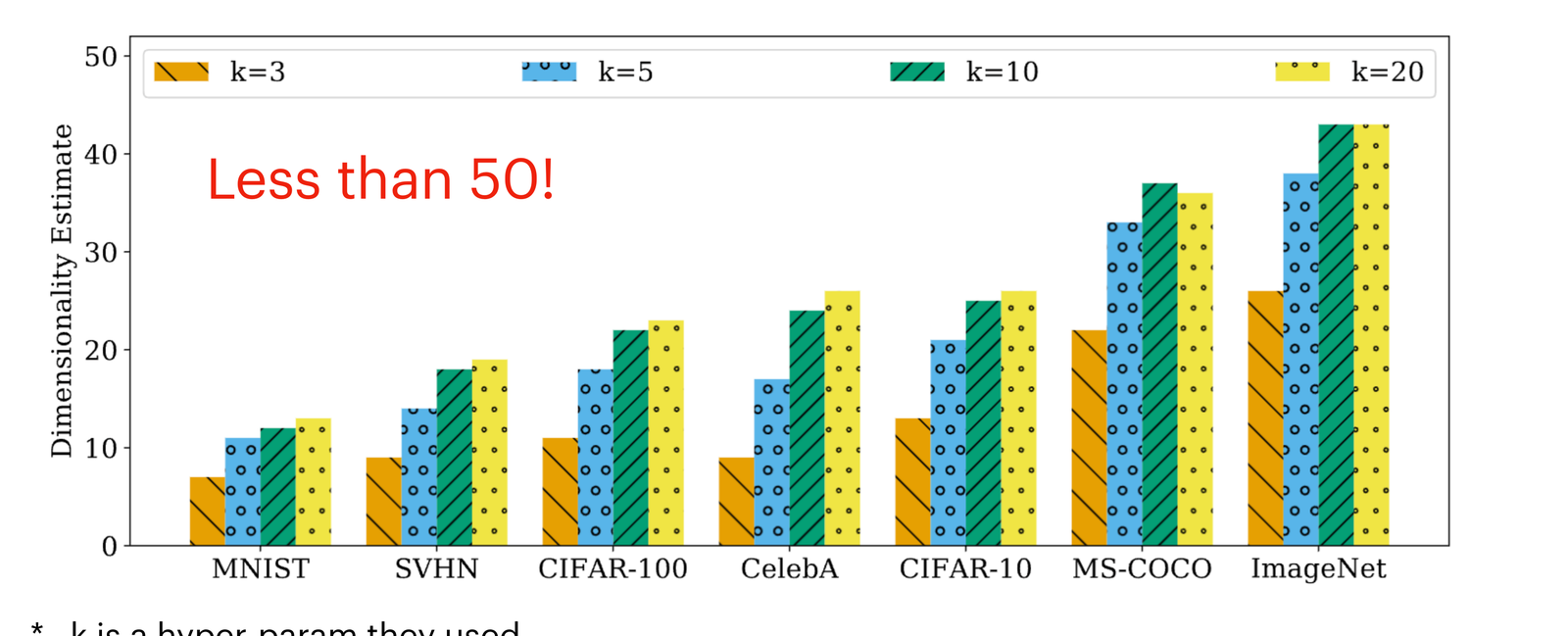
The punchline deserves restating: ImageNet, with its 150,528-pixel ambient space, has an intrinsic dimension below fifty. Almost all of pixel space is empty of natural images.
Why the number matters
Task difficulty tracks dimension
Sorting datasets by estimated dimension reproduces the folk ordering of their difficulty. State-of-the-art accuracy falls as intrinsic dimension rises, even when training set sizes differ by orders of magnitude:
| Dataset | MNIST | SVHN | CIFAR-100 | CelebA | CIFAR-10 | MS-COCO | ImageNet |
|---|---|---|---|---|---|---|---|
| MLE ($k$=3) | 7 | 9 | 11 | 9 | 13 | 22 | 26 |
| MLE ($k$=5) | 11 | 14 | 18 | 17 | 21 | 33 | 38 |
| MLE ($k$=10) | 12 | 18 | 22 | 24 | 25 | 37 | 43 |
| MLE ($k$=20) | 13 | 19 | 23 | 26 | 26 | 36 | 43 |
| SOTA accuracy | 99.84 | 99.01 | 93.51 | – | 99.37 | – | 88.55 |
Generation difficulty scales the same way. For diffusion models under the manifold hypothesis, Potaptchik et al. [3] show the number of diffusion steps required for sampling grows as $O(d)$ in the intrinsic dimension $d$, linking the geometry directly to inference cost.
Guidance for generator design
The number also reads as a design constraint. When the latent space of a generator is far wider than the data manifold, training pays for the mismatch. The StyleGAN-XL authors [4] reached the same conclusion from the practical side:
Accordingly, a latent code of size 512 is highly redundant, making the mapping network’s task harder at the beginning of training. Consequently, the generator is slow to adapt and cannot benefit from Projected GAN’s speed up. We therefore reduce StyleGAN’s latent code $z$ to 64.
Sauer, Schwarz, and Geiger, StyleGAN-XL
A latent width of 64 sits comfortably above the measured intrinsic dimension of ImageNet while discarding hundreds of redundant coordinates.
Detecting AI-generated text
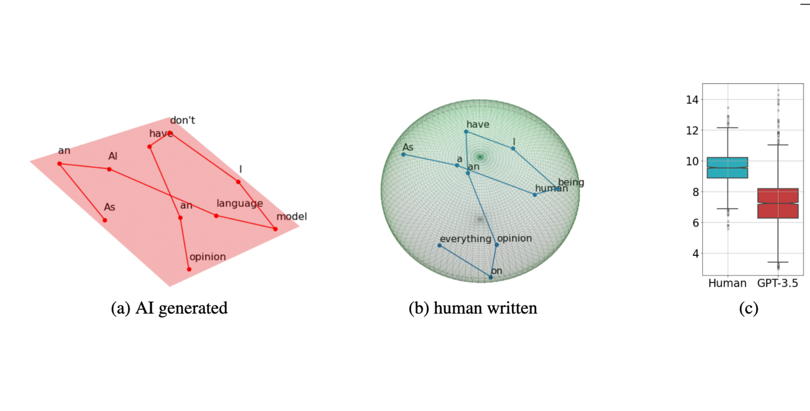
Intrinsic dimension separates sources of text, not just images. Tulchinskii et al. [5] estimate the dimension of contextual embeddings and find human-written text consistently measures higher, around 9 to 10, than GPT-3.5 generations, around 7 to 8. The gap is stable enough to power a detector that holds up across domains and models.
One number, estimated from nearest-neighbor distances alone, predicts classification difficulty, prices generative sampling, sizes latent spaces, and flags synthetic text. Worth knowing for your data.
References
- Elizaveta Levina and Peter J. Bickel. Maximum likelihood estimation of intrinsic dimension. In Advances in Neural Information Processing Systems, 2004.
- Phillip Pope, Chen Zhu, Ahmed Abdelkader, Micah Goldblum, and Tom Goldstein. The intrinsic dimension of images and its impact on learning. In ICLR, 2021.
- Peter Potaptchik, Iskander Azangulov, and George Deligiannidis. Linear convergence of diffusion models under the manifold hypothesis. 2024.
- Axel Sauer, Katja Schwarz, and Andreas Geiger. StyleGAN-XL: Scaling StyleGAN to large diverse datasets. In ACM SIGGRAPH, 2022.
- Eduard Tulchinskii, Kristian Kuznetsov, Laida Kushnareva, Daniil Cherniavskii, Sergey Nikolenko, Evgeny Burnaev, Serguei Barannikov, and Irina Piontkovskaya. Intrinsic dimension estimation for robust detection of AI-generated texts. In Advances in Neural Information Processing Systems, 2023.